
The process is used to find a more direct route between two points along a surface. The process takes a user drawn line (path) over a raster (representing either a 3D surface raster or a cost raster) and then iteratively figures increasingly shorter and shorter paths.
Depending on the type of surface, distance is figured in either 3D space (with an elevation raster) or 2D space (with a cost raster). You can apply a relative to the Z distance when using an elevation raster. Movement from the initial line (and each subsequent path) can be restricted by increasing the parameter. Accuracy can be increased by increasing the number of (steps per cell).
The process continuously loops to converge on the shortest path, however, it can not be expected that an optimal solution will be reached in a reasonable amount of time — or ever. Thus the process is designed for you to stop it at any time and still retain the line generated by the last iteration.
Prerequisite Skills: Displaying Geospatial Data and TNT Product Concepts.
Sample Data: coolumbooka.zip
(A portion of a 2 meter DEM from NSW FSDF was extracted to fit within the size constraints of the TNTmips Free license level.)
Tutorial Lesson: One exercise gives quick introduction (see below).
To run the process: select the input, draw a line in the , and click .
Notice the new vector is automatically added to the .
For the following steps, experiment with adjusting the parameters and/or the initial line then re-run the process between each change. Use and at your discretion.
Notice, increasing slows down the processing speed.
If you save to a vector, you can verify the number of knots per cell by zooming in on part of the resulting path (i.e. view scale of 1:100). Optionally turn on: to more easily see raster cell boundaries.
Notice how increasing the restricts movement of the line away from its initial path.
The process takes a single raster as input (signed/unsigned integer: 8-, 16-, and 32-bit; floating: 32- and 64-bit). Raster cells can contain a surface elevation or cost value and this determines how to figure the distance (via setting).
- Computes the shortest path based on distance in 3D space. With this method, the raster cell values represent elevation and you can specify a value to amplify or reduce the vertical distance (Z direction) relative to the horizontal distance (on the XY plane). In other words, increase the exaggerate the vertical distance.
- Computes the shortest path based on the path length in 2D space multiplied by the cell value. Here the cell value represents the cost of traveling through the cell (i.e. price per acre, distance to population center, flood zone).
Tip: see the Multi-Criteria Decision Analysis Tech Guide for information on how to create a cost raster.
The initial path is manually drawn in the window using the drawing tool. This is the starting path for the first iteration and thus influences each subsequent iteration. Intermediate vertices in the starting path affect the way maximum permissible elevation changes constrain changes to the path. So different paths between the same two points will converge on different solutions.
Tip: a high will prevent drastic changes to the initial line. Increasing the will exaggerate surface distances.
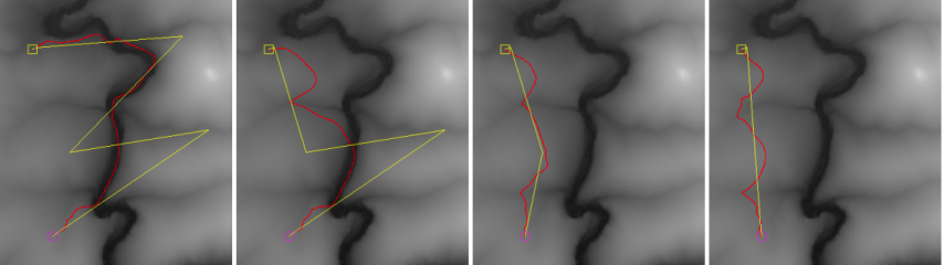
As the process iterates, the current path is updated and displayed in the . You can stop the process at any time and save the current results. You will find that sometimes the path will change and converge on a final solution rapidly. Other times it continues to run without making significant changes to the path. The process will stop automatically if and when a final solution is found. However, if it does not find a solution quickly, a window opens with a button you can use to finish it manually.
After the process is stopped you have the option of saving the current result and/or running the process again (i.e. with adjusted parameters and/or a new or modified prototype line).
If you use to save the current line to a vector object, it is automatically added to the as a vector layer.
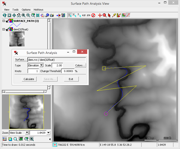
The dialog and the window are used to run the process. This document refers to dialog as the 'main process' window and window as the .
window.
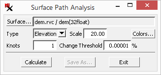
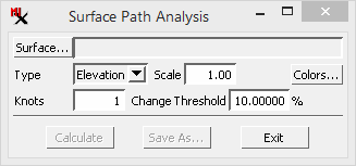
- Select an elevation or cost raster.
- Specify the type of raster you chose for the surface: or . The option activates the parameter, however, the option will not take the value into account.
- Steps per cell. The number of knots is used to determine how many steps along
the line are used to define the path. A step is equal to cell size
divided by the number of knots. Possible values are between 1 and 16. The larger the number of knots, the
smaller the step. Increasing the number of knots will increase the time it takes the
process to complete, however, it provides more accuracy.
Tip: Start with a setting of :1 (one step per cell) to see the quickest result.
- The Scale value lets you set a ratio for horizontal (Z) movement to the vertical (XY) movement. Possible values are between .01 to 1000. As the is increased, the more vertical movement is emphasized. For example a value of 2 means up and down movement is emphasized over horizontal movement by a scale of 1:2 (horizontal:vertical). On the other hand, a of .01 (1:.01) results in a straighter line because horizontal movement is amplified.
- Set a threshold for the percentage of change allowed. Possible values are between .00001 to 10.00000. If the new path is not shorter than it by the percentage specified, the processing will automatically stop. Raising this value restricts line changes while lowering it allows more drastic differences.
See the Introduction to the Display Interface for more information about the typical features and tools in the window. An additional tool is added for the process and is described here.
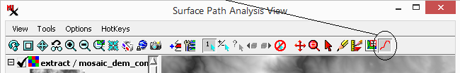
![]() Line -
Use the Line tool to draw the line for the prototype path that the process start with. With the Line tool selected, draw a line by clicking at positions on the View window to define the starting, intermediate, and ending vertices. Click the right mouse button (or in the main dialog) to accept the prototype line element and start processing.
Line -
Use the Line tool to draw the line for the prototype path that the process start with. With the Line tool selected, draw a line by clicking at positions on the View window to define the starting, intermediate, and ending vertices. Click the right mouse button (or in the main dialog) to accept the prototype line element and start processing.