TNTmips offers a variety of tools that work along with a user drawn element (i.e. point, line, or polygon) in the window. Some tools are used to create a sketch or region object and others let the user specify an area for processing.
There are two drawing modes that determine whether you can use click–and–drag to draw a curved line () or not ().
mode – Allows drawing curves. The drawn line follows the cursor path when you click–and–drag the mouse. It also lets you use a series of clicks (no drag) to add straight segments.
mode – Restricts drawing to straight line segments. Vertices are added for each mouse click with straight line segments between them.
TAB key – Use the TAB key on your keyboard to switch between the two drawing modes.
After drawing a prototype line or polygon, you can edit it by moving, adding, and deleting vertices. A prototype line is drawn in the with special symbols for the start and end nodes. Furthermore, moving the mouse near the line activates symbols to indicate whether you are near an existing vertex or not. These symbols give you cues to help you edit the prototype line/polygon:
square box symbol – A square box is always shown around the starting node.
circle symbol – A circle is always shown around the ending node.
plus sign symbol – Indicates there is a vertex on the line at the current mouse location. Shows only when mouse is near a vertex. When this symbol is shown, you can click–and–drag to move the vertex.
diamond symbol – Indicates a position on the line where there is no vertex. Shows only when mouse is over a line position with no vertex. When this symbol is shown, you can click to insert a vertex.
DELETE key – Move your mouse over a vertex and click the DELETE key on your keyboard to remove that vertex.
ESCAPE key – Click the ESC key on your keyboard to clear the prototype element.
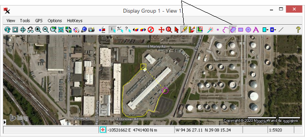
The normal order of operations is to select the tool, draw an element, and either save your drawing or apply an operation to the drawn element. With some tools you also need to choose the type of element to draw (i.e. point, line, polygon). While this example uses the tool, many of the steps are common to other drawing tools.
Open the process and add a reference layer.
When you select the tool several icons will appear to the right of it including several options for the type of element you want to draw. Widen the window if you don't see all of the icons.
Notice the starting vertex is indicated with a square around it and the last vertex drawn has a circle around it.
Notice it is now restricted to drawing only straight line segments
After inserting a vertex, notice the cursor changes to a plus (+) so you can drag it to adjust the position.
Notice in this example the right–mouse button adds an element to a Sketch object. With other drawing tools the right–mouse button may open a menu for you to select another action.
Tip: if you make a mistake while drawing, press the Escape key to clear the prototype element.
A geospatial data item may be a raster, vector, shape, CAD, LiDAR, TIN, database, or region structure. The following shorthand terms have important distinctions when describing geodata in TNTgis. Simply put: items are stored in your computer (in files or RVC objects) versus displayed in TNTmips (as layers).
file – An item in a drive or folder of your computer — in particular, geodata files such as GeoTIFF (.tif), shapefile (.shp), and RVC (.rvc) files. Most geospatial file formats contains a single raster, vector, shape, CAD, LiDAR, TIN, database, or region structure. However, some file formats support multiple co–aligned raster bands. Other formats can contain multiple geodata items as well as different types of geodata structures (such as .rvc).
object – A geospatial item within an RVC file is called an object. An object may be a raster, vector, shape, CAD, LiDAR, TIN, database, or region structure.
layer – A geospatial file or object added to a TNTmips process for display. Typically one file or object is used in each layer, however that is not always the case since raster layers can be made up of multiple bands.
TNTgis supports importing and exporting an unsurpassed number of external geospatial file formats to/from the RVC format. The TNTgis proprietary RVC file format is a unique container for geospatial data in raster, vector, shape, CAD, LiDAR, TIN, database, and region form.
In addition, TNTmips processes support direct use of some external formats. For example, you can directly display files in these popular formats: GeoTIFF, JPEG2000, PNG, MrSID, ECW, shapefile, File Geodatabase, Oracle Spatial, DGN, TAB, DXF, DWG.
See also: Geodata Formats and Geodata Format Summary Table
RVC file (.rvc) – The proprietary RVC file structure allows for the creation, modification, and storage of geospatial data of various kinds (i.e. rasters, vectors, CAD, and database data). Within TNTmips the RVC file acts as a folder where you can keep a collection of various geodata 'objects'. Some people use RVC files to keep related geodata together. Others prefer to store only one geospatial item per RVC file.
RVC object – Items within an RVC file are called objects, however, conceptually these objects are like 'files' within an RVC 'folder'. For example, you may import a geospatial data file (such as GeoTIFF or shapefile) to an object within an RVC file.
A raster data structure is a two–dimensional array of cells containing numbers of a single data type (i.e. rows and columns of numbers).
A photograph is a simple example of a raster, however, in TNTgis a raster usually represents an area on the ground. Thus each cell in a raster can hold a number that represents a measurable characteristic in the corresponding area of space such as: spectral reflectance, image color, brightness, greenness, elevation, type of ground cover, or chemical concentration values.
Raster cell values can be a continuous range such as when created by a camera or other sensor, or values may be arbitrary numbers such as to represent ground cover class or a color in a color palette.
Rasters are especially useful because image traits are represented numerically (raster cell values) and cells are organized in a uniform grid with equal areas. These two qualities make numerical and display computations very fast and straightforward, even though different raster objects can represent diverse image characteristics.
raster data type – Also referred to as bit–depth. Indicates the number of storage bits used to hold the number in each raster cell and whether the number is signed or unsigned. Raster object cells can have data types of 1–bit (binary), 4–bit, 8–bit, 16–bit, 32–bit, or 64–bits of either integer or real numeric values. It restricts the range and type of values that can be stored in the cells of a raster.
The raster data type also indicates whether the file or object contains a single raster or a composite raster set such as three band values stored in 16–or 24–bits (RGB, BGR) or four band values in 32–bits (RGBA, ARGB, CMYK, KCMY). In addition, a raster data type can be 64– and 128–bit complex numbers (R/I, M/P).
composite raster – may refer to how co–aligned rasters are stored together (in composite raster file) or how they are displayed (as composite color layer).
composite raster file / object – a composite raster file contains multiple raster bands in a single file. The same is true for composite objects.
co–aligned rasters – rasters that overlay each other perfectly in terms of geographic extent, cell size, and number of rows/columns.
Tip: Use the Resample using Georeference process to resample lower resolution images so they are co–aligned with the higher resolution raster. (Set higher resolution image as: Reference Raster and then set Extents and Cell Size to Match Reference.)
There are three general ways to display a raster: as a grayscale layer, indexed color with palette, or as a composite layer using a color mode. All three methods can be displayed with or without contrast enhancement, which lets you adjust the cell value range for optimal display intensity. The data type of the raster(s) you want to use determine the type of raster layer you can add.
composite layer / composite color / composite color layer – indicates how a layer with multiple co–aligned raster bands is displayed. Composite layers are added by first choosing the color mode and then the bands for each component. The raster cell values for RGB layers are directly displayed. Non–RGB composite layer modes are emulated in the display by first converting raster values to RGB values.
Supported color modes include the following three or four band layers: RGB (Red–Green–Blue), HIS (Hue–Intensity–Saturation), HBS (Hugh–Brightness–Saturation), RGBI (Red–Green–Blue–Intensity), CMY (Cyan–Magenta–Yellow), and CMYK (Cyan–Magenta–Yellow–Black).
Composite layers may be set up using bands stored in one file (or object) or in separate files (or objects). For example, an RGB layer may be made from bands stored in one file or from three separate grayscale raster files.
RGB layer (Red–Green–Blue) – a composite layer with three separate raster bands to specify intensity values for each of the three display color components (Red, Green, and Blue). A display monitor has the same three RGB color components that are used to display colors.
CMYK layer (Cyan–Magenta–Yellow–Black) – a composite layer with four separate raster bands: Cyan, Magenta, Yellow and Black containing values in the CMYK color mode. CMYK values are converted to RGB color to emulate CMYK colors in the display. (The CMY model is used for producing color by mixing or overlaying translucent filters or inks, as in printing. Thus it isn't directly supported in a display monitor.)
multiband layer – a composite layer that can include all of the raster bands in a scene and is typically used for multispectral data. Since all the bands in the layer are available, you can easily change which of the three bands are assigned to the RGB color components used to display it (via in ). Compare this to an RGB layer that lets you adjust only the three bands initially selected.
Tip: open Raster Layer Controls for the multiband raster layer and specify a raster for each color component (Red, Green, Blue) in the Object tab. Then verify Contrast is identical for each color component (i.e. Auto Normalize).
grayscale layer – the range of cell values are spread between black (0 cell value) and white (255).
index color with palette (color map) – an 8–bit raster set up with a color palette containing 256 colors. Rasters with higher than 8–bit data type can also use indexed color but must first use contrast enhancement to reduce the number of raster values to 8–bits (256 values). (A 4–bit raster/color palette is also supported.)
hyperspectral layer – A composite layer with many input bands optimized for use with hyperspectral data in the process. As with multi–band layer, the user can set which three bands are used to display it in the RGB color mode.
In most cases you can use to quickly add a raster layer. However, since there are many ways to store raster data and display raster layers, the menu gives you more options and control when setting up composite raster layers.
– This method has the user choose the input raster or rasters and the layer is automatically added. It is a quick and straight–forward way to add most geodata layers including raster layers. Use this method to:
– This method opens a menu that lets you choose the type of raster layer you want to add and then prompts for the needed raster bands. Use this option to:
contrast enhancement – If the raster data type is more than 8–bits, contrast enhancement is used to adjust the input cell value range to an 8–bit range for display purposes. This may apply to grayscale, color with palette, and RGB (or other composite) layers.
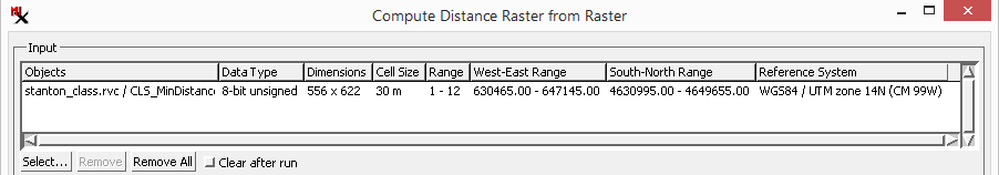
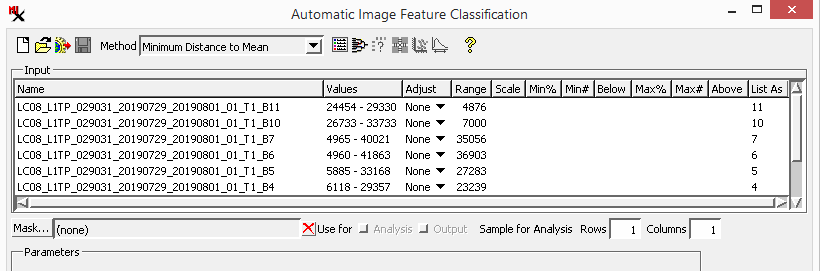
Image processes that allow multiple input rasters may show the selected input in a list where each raster is in its own row. This list includes columns with information about each raster such as:
object name, , cell value , and coordinate . Columns that are shown by default may be of particular use in the process. Columns may be process–specific or universally useful.
Right–click on a column headings to see a menu with options to sort the list () and automatically adjust the column width (). Some processes have a option that opens a dialog for you to specify what columns to show.
Click on a row to select a raster. In some processes there are tools that work with the selected input raster and/or let you remove the selected raster from the list.
selected input rasters with default columns for that process.
columns such as and .
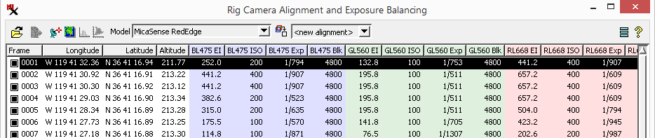
additional columns with EXIF information that is useful in the process.
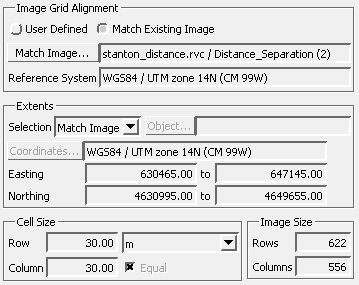
Processes that create rasters (or extract a portion of a raster) have settings that let you specify the new raster structure called the raster grid.
raster grid – is made of of the rows and columns of raster cells. It includes the coordinate reference system and alignment to it as well as the cell size, number of lines/columns, and geographic extents.
There are four secions in the raster grid controls: , and .
used to
easily and automatically
set up the complete raster grid.
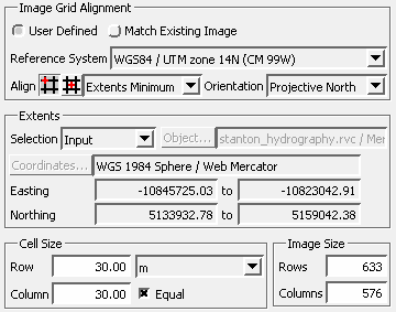
The pane has options for aligning the raster to the Coordinate (CRS).
– lets you select an existing raster to make the output raster structure. This is a quick and accurate way to set up the entire raster grid, extents, and CRS.
– lets you manually set the alignment by making the and settings available.
– includes two settings that determine exactly how the raster is aligned with the CRS. One setting is the position within a cell to tie to (corner or center). The other is the alignment method and may include setting a particular CRS coordinate to a specific raster cell. This is similar to what is set up for a simple georeference in the process. Note, this setting is available only when the option is on.
First select the cell position to align to:
![]() – aligns to the outer corner of the cell.
– aligns to the outer corner of the cell.
![]() – aligns to the center of the cell.
– aligns to the center of the cell.
Then choose the alignment method. In most cases, use the default option to automatically align to the CRS grid. Alternatively, align one of the coordinates (specified in the section) to the corresponding raster corner cells.
– aligns cells to the CRS.
This option is directly related to the cell size and results in map coordinates that are an integral multiple of the cell size.
I.e. if the cell size is 7 meters and is set to , the raster cell corner coordinates will be an integer multiple of 7.
– extents coordinate at lower left of image to align with lower left cell of the output raster.
– extents coordinate at upper right of image to align with upper right cell of the output raster.
– of the raster grid to , or . Note, this setting is available only when the option is on.
The pane has options for setting the coordinate range of the raster. You can independently set the extents even if the option in the pane is used. The options determines the method used to set them:
– a user entered range for and (or and ) values. When this option is set, use the field to set the CRS you want to use for the manually entered coordinate range values. (The four values entered also define the four corner coordinates.)
– lets the user select a geometric object to match the extents to.
– uses the input object's extents.
– this option is the default option if the option in the pane. If set here, that raster will specify the extents as well as the image grid alignment and cell size.
The and panes have options for setting the raster's cell size via the and settings as well as the number of and in the raster. The cell size and image size settings are tied to each other. When one is changed the other is automatically adjusted to fit the raster extents.
These options are set automatically if the option in the panel is set. They can be manually set when the option is used.
When using geometric objects or files, some processes let you select which elements you want to process using the options below.
– all elements in the object or all elements of the specified type are used.
– this option activates the button, which opens the window with the typical methods available to mark elements: tool (icon) in , (select or by region methods), (and other mark options for element databases in the ), and in some cases the sidebar tool (with a corresponding tool icon at the top of the window).
– select by query. See the Mark / Show Elements by Query section for information on how to select elements using associated database records.
In addition, elements in vector objects may be selected by element type (point, line, or polygon).