
The TNTmips® process automatically groups image cells with similar spectral properties into classes. This process uses the spectral pattern (or "color") of a raster cell in multispectral or multi-temporal imagery to automatically categorize all cells into spectral classes. The relationship between spectral classes and different surface materials or land cover types may be known beforehand or determined after classification by analysis of the spectral properties of each class.
The process offers a variety of classification methods as well as tools to aid in the analysis of the classification results. Unsupervised methods automatically group image cells with similar spectral properties while supervised methods require you to identify sample class areas to train the process. After running the classification process, various statistics and analysis tools are available to help you study the class results and interactively merge similar classes.
Prerequisite Skills: Displaying Geospatial Data and TNT Product Concepts.
Sample Data: stanton.zipThe first three lessons provide a quick introduction. Unless otherwise indicated, subsequent lessons can be done in any order independently from the reading.
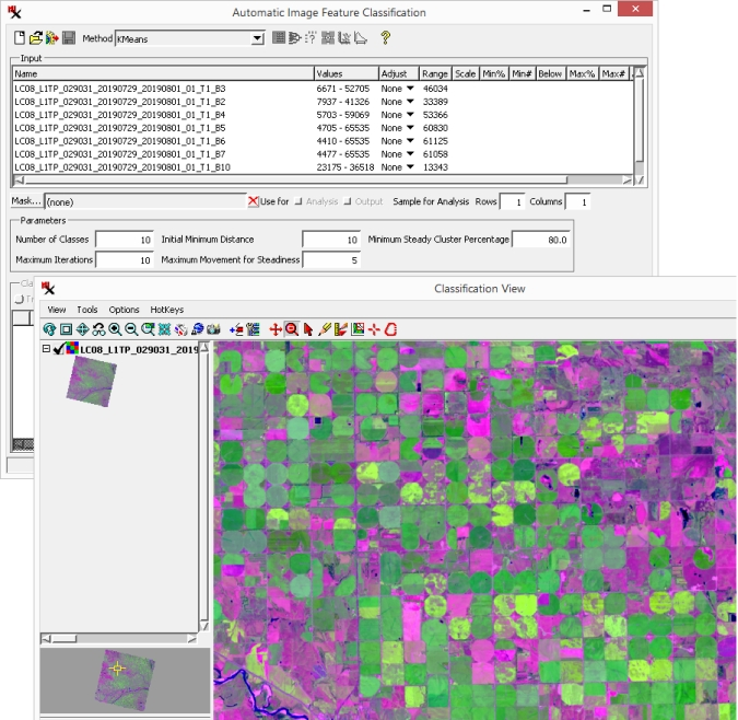
To try a quick run through of the process all you need to do is select the input, choose an unsupervised classification method, set the number of classes, and run it.
Make a note of the file path and name of the output .rvc file where you put the class and distance rasters. You can re-load the resulting class raster using the icon to use the same results in later exercises.
(continued from previous exercise)
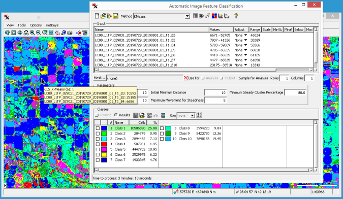
After the classification is finished running the resulting class raster is automatically loaded in the window.
(continued from previous exercise)
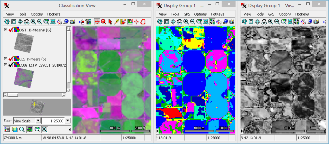
Zoom in to an area of interest, then use the checkbox for layers in to compare the input rasters with the resulting class and distance rasters.
The following steps are done in the window.
The default name of the distance raster begins with "DST" followed by the name. If the distance raster displays too dark, set the layer's to (via ![]() Raster Layer Controls).
Raster Layer Controls).
Tip: if the value set for the is too small you may notice some classes contain more than one ground feature. However, a small number of classes is simpler to manage when first learning to use the tools to analyze classes in later exercises.
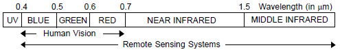
Many remote sensing systems record brightness values at different wavelengths that commonly include portions of the visible light spectrum as well as photoinfrared and middle infrared bands. The brightness values for each of these bands are typically stored in a separate grayscale image (raster). Each cell in a multiband image therefore has a set of brightness values which in effect represent the "color" of that patch of the ground surface. (Here we extend our concept of color to include wavelengths beyond the visible light range.)
spectral space - An N-dimensional space where N is the number of input rasters with each on their own coordinate axis.
spectral pattern - Coordinates of a point in spectral space. In other words, the values taken from all the input rasters for a single raster cell. Consider viewing an RGB layer made up of three bands. The red, green, and blue values for a single image cell are used when displaying it in color. In spectral space, these values make up the spectral pattern for a point.
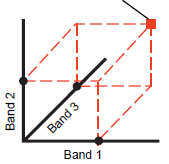
The spectral pattern of a cell in a multispectral image can be quantified by plotting the raster values from each band on a separate coordinate axis to locate a point in a hypothetical spectral space. Most classification methods use some measure of the distance between points in this spectral space to assess the similarity of spectral patterns. Cells that are close together in spectral space have similar spectral properties and have a high likelihood of being the same surface feature.
Select multiple rasters covering the same ground area for the process input such as multispectral bands, hyperspectral bands, or multi-temporal data. A single raster is also allowed. The input rasters ...
Tip: you do not need to scale the input ranges before using them. You can adjust the cell value ranges directly in the process if needed.
Ground truth data containing any available information about the types of materials and ground cover in the scene is useful but not required. It could be a map with hand drawn feature areas or a raster with high enough resolution that you can recognize features. Any type of ground truth data that is georeferenced can be manually added to the as a reference layer. Such a reference layer may be used in both unsupervised and supervised classification to compare the resulting class raster to ground truth information.
Ground truth data can also be used to create the required training set raster for use in supervised classification. Vector polygons or points containing class attributes can be imported directly to a training set raster. Reference layers can be added to the and used to manually create a training set raster.
A binary raster can be used to eliminate areas for processing and/or to set areas as null in the resulting class raster. A mask may be useful depending on your data but is not required. The Automatic Classification process is influenced by the brightness values of all cells in the scene, not just the features that you intend to classify. Thus using a mask to eliminate unwanted areas can vastly reduce the number of classes needed to differentiate materials in the area of interest.
The mask raster must be co-aligned with the input bands. Cell values of 1 in the binary raster will be processed while 0 values will be masked.
The primary classification result is a class raster, which is automatically displayed in a View window after running the process. For clarity, we call this the raster in this document. Some classification methods also give you the option of creating a distance raster, which you can manually add to the .
class raster - a categorical 8-bit unsigned raster where each (arbitrary) numerical value in the raster represents a class that is assigned to the cell by the classification process. The raster includes a color palette, used to display the layer, with a color assigned to each cell value.
results raster - the currently loaded class raster. After running the process, the resulting class raster is automatically loaded and ready for analysis.
distance raster - a 32-bit floating point / grayscale raster that shows how well each cell fits its assigned class. Each raster cell value records the distance between that cell and its class center in spectral space. Cells that are closer to their class center (better fit) appear darker in the displayed raster than those with greater distance values (poorer fit).
In addition, statistics and class analysis data is produced along with tools to help you study the resulting classes: the and windows can be saved to standard text or CAD file formats.
The dialog and the window are used to run the process. This document refers to dialog as the 'main process' window and window as the .
![]()
The left-most options let you setup and run the automated classification process:
![]() New - Click the icon to select a set of input rasters to be classified.
New - Click the icon to select a set of input rasters to be classified.
![]() Open - Reopen a previously made class raster to automatically load it with input rasters and settings.
Open - Reopen a previously made class raster to automatically load it with input rasters and settings.
![]() Run - Run the image classification to create a class raster.
Run - Run the image classification to create a class raster.
- Click the drop down list to choose from a menu of classification methods. The list is ordered so that Unsupervised Methods are above all of the Supervised Methods. Note the toggle in the section becomes active if a supervised method is selected.
The top right options (in top toolbar) open statistics and analysis tools for evaluating classes.
![]() Statistics and
Statistics and
![]() Classification Dendrogram are available for both class results ( mode) and training classes ( mode).
Classification Dendrogram are available for both class results ( mode) and training classes ( mode).
![]() Confusion Matrix,
Confusion Matrix,
![]() Cooccurrence,
Cooccurrence,
![]() Scatterplot, and
Scatterplot, and
![]() Distance Histogram are available only after running the process (in mode).
See the Analyze Classes section for details about these statistics and analysis tools.
Distance Histogram are available only after running the process (in mode).
See the Analyze Classes section for details about these statistics and analysis tools.
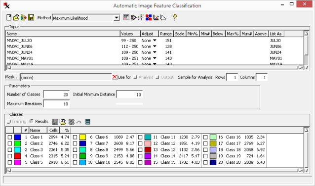
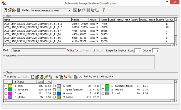
- Selected input rasters are shown in a scrollable pane. , and columns can be used to adjust the input raster's cell value range. , and specify how to handle values outside of the adjusted range.
- Shows the name of the input raster.
- Shows the input raster cell value range.
- Method used to adjust input range: .
Use this setting to ensure that a "difference" in adjusted DN values has the same statistical significance in all of the bands.
Otherwise, the multi-band statistics for some classification methods will be biased and may separate or combine classes in undesired ways —
such as when the values are dispersed much more in some bands than in others. For typical satellite imagery with either TOA reflectance or ground-corrected reflectance,
there is usually no need to use the Adjust setting.
However, if multimodal classfication is done, such as mixing aeromagnetic, radar, and electro–optical (visible – nir, etc.) then rescaling can be important.
- The initial default for the linear rescaling range is the difference between highest and lowest adjusted cell values.
You can manually set it (unless is set to )
and the will be automatically adjusted.
- Value use to scale the input. In order to manually modify , set .
Changes to the or automatically adjust each other.
- Shows the percentage of values below the .
- Shows the lowest number in the range of adjusted values.
- Specify how to handle values below the : .
- Shows the percentage of values above the .
- Shows the highest number in the range of adjusted values.
- Specify how to handle values above the : .
- Set the name shown in .
Typically you can use the input without any scale adjustments. However, if you are mixing input from different sources you may have significantly different cell value ranges, which would result in some rasters having more influence on the classification than others. You can apply a scale to any input raster to make the cell value ranges more similar and thus remove any bias.
The process plots input cell values and computes distance in Euclidean space and this is used to classify cells. Thus a difference of '1' between cell values in a raster with a wide range is given the same emphasis as a raster with a narrow range of cell values. For example, a floating point raster with a cell value range between 0 and 1 would have a distance less than 1 between all cell values. Thus there will be no difference between them in Euclidean space. You can correct for this by applying a scale to broaden the cell value range. To think of it another way, if you want to emphasize an input raster, spread out its cell value range relative to the other input rasters.
- Select a binary raster to mask out areas of the scene you don't want processed for and/or . Cell values of 1 in the binary raster will be processed while 0 values will be masked. The mask raster must be co-aligned with the input bands.
- Removes the mask raster.
- Used if a is selected. Choose and/or to specify the areas to process. Use the option to ensure the set of classes is determined using only the unmasked areas. This can significantly reduce the number of classes needed and still separate the features in the areas of interest. Use the to create classes only for your area of interest. In that case, the resulting class raster will have null areas matching the mask binary raster.
- Sets the classification to build classes from a subset of the input image cells before applying the classes to the entire image. Sample cells are selected at regular intervals throughout the image. Set the sampling intervals for both and . The default settings of 1 ensures all input cells are used to build classes. Increasing these values speeds processing for large images. For example, changing both intervals to 2 results in a sample set made up of one quarter of the image cells.
The settings in the panel are dependent on the selected. See the Unsupervised Methods and Supervised Methods sections for information about each method and their parameters.
The classes and toolbar options shown in the panel are dependent on the mode selected — mode or mode.
mode - Uses the resulting class raster and shows its class list below. This mode has a special toolbar with options you can use to modify the classes and save your changes.
![]() Save Results - Use to save the class raster after modifying classes. It is available after running the process and overwrites the current class raster without prompting. Note, after saving you can no longer merged/modified classes.
Save Results - Use to save the class raster after modifying classes. It is available after running the process and overwrites the current class raster without prompting. Note, after saving you can no longer merged/modified classes.
![]() Save Results As - Saves the updated classes to new class raster.
Save Results As - Saves the updated classes to new class raster.
![]() Merge Selected Classes,
Merge Selected Classes, ![]() Undo, and
Undo, and ![]() Settings - See the Merge Class section.
Settings - See the Merge Class section.
mode - Lets you set up and work with a training set raster required for supervised classification. Shows list of training classes and includes a toolbar with options to create and work with them. See the Training Set section for more information on the following options available in this mode:
![]() New Training Data,
New Training Data,
![]() Open Training Data,
Open Training Data,
![]() Save Training Data As,
Save Training Data As,
![]() Edit Training Data,
Edit Training Data,
![]() Import,
Import,
![]() Open Class Table,
Open Class Table,
![]() Save Class Table,
Save Class Table,
![]() Add Class,
Add Class,
![]() Delete Selected Class,
Delete Selected Class,
![]() Apply Cell Value Changes, and
Apply Cell Value Changes, and
![]() Reset Cell Values as Saved.
Reset Cell Values as Saved.
classes list - If mode is on, the classes created after running the process are shown. If mode is on, it shows the training classes.
selection box - Click the box on the left side of a class cell value to select or unselect it. The selected class(es) can be used in various ways. For example, the selected class is used along with the tool in the to set up training areas in a training set raster. Selected classes are also highlighted in the analysis tool windows to help you study the resulting class raster. Furthermore, if two or more classes are selected, the icon becomes available and a single selected class will be used to specify the class when you open the .
- This number indicates the cell value in the class raster.
color sample - Color used to display the class in the View window. Click the color sample to open controls to change it.
- The name of the class. Double-click the name to change it.
- The number of image cells in the class.
- Percentage of cells in that class.
See the Introduction to the Display Interface for more information about the typical features and tools in the . Special tools for the process are listed below.
![]()
In addition to the normal features and tools, there are two tools you can use to create and modify a training set class raster. These tools are closely tied to the class or classes selected in the main process window ( mode only).
![]() Select Class - This is a shortcut to select and unselect classes and thus lets you avoid having to move your mouse between the and main process windows. Simply click on a feature (raster cell) in the that has a class assigned to it — this toggles the selection box for that class in the main process window.
Select Class - This is a shortcut to select and unselect classes and thus lets you avoid having to move your mouse between the and main process windows. Simply click on a feature (raster cell) in the that has a class assigned to it — this toggles the selection box for that class in the main process window.
![]() Select Area - Lets you add training samples to the training set raster. Draw a polygon around a ground feature and then right-click to open a menu with commands to perform on the selected cell(s). See the Add Samples to a Training Set Raster section for more details on the following commands:
,
,
,
,
,
,
.
Select Area - Lets you add training samples to the training set raster. Draw a polygon around a ground feature and then right-click to open a menu with commands to perform on the selected cell(s). See the Add Samples to a Training Set Raster section for more details on the following commands:
,
,
,
,
,
,
.
In unsupervised classification, TNTmips uses a set of rules to automatically find the desired number of naturally occurring spectral classes from the set of input rasters. The rules vary depending on the classification method you choose from the Method option menu. Unsupervised methods do not require training data.
An unsupervised classification assigns class numbers in the order in which the classes are created. Because the raster values have no other numerical significance, for display a unique color is assigned to each class from a standard color palette.
Note that unsupervised methods are listed first in the list followed by the supervised methods.
The following unsupervised classification methods are available:. See the Unsupervised Methods and their Parameters section for details on each method.
Start where the previous lesson left off or load any input. [I.e. re-load the class raster resulting from the first exercise (via icon) to quickly set up input rasters.]
Previous exercises used the unsupervised method.
Tip: when you perform an unsupervised classification, set the number of output classes to be several times greater than the number of land cover types that you hope to recognize. You can then use the available analysis tools to recognize and merge similar spectral classes.
A typical workflow in an unsupervised classification involves creating more classes than you need, looking at the class statistics such as cooccurrence and separation, and then manually merging classes that you've determined are the same material. The next section has information on how to Analyze Classes. For now we will skip the analysis step and focus on steps to merge. The section of the main process window provides a simple interface for interactively merging two or more classes.
![]() Merge Selected Classes - Merges the (two or more) selected classes into one class.
Merge Selected Classes - Merges the (two or more) selected classes into one class.
![]() Undo - Reverts last set of merged classes back to original classes. Use multiple times to undo all previous operations.
Undo - Reverts last set of merged classes back to original classes. Use multiple times to undo all previous operations.
![]() Settings - for merging classes
Settings - for merging classes
- When on, classes are renumbered to avoid gaps in the cell value numbers (#).
- When on, a merged class is given a new color sample created by mixing the original class color samples. Otherwise one of the selected class colors is used.
Get familiar with the interactive tools for merging classes. (This exercise skips the step of studying the classes to determine which, if any, need to be merged.)
Start with a previous run of the process loaded so you see a class raster and classes listed. (I.e. load the class raster resulting from the first exercise.)
After running the process, the resulting class raster ( raster) is automatically loaded. Or, add a previously created class raster to automatically reload all input bands and recalculate class statistics and analysis data. Either way the raster is ready for analysis. An array of tools are available to help determine if the classes sufficiently represent the ground materials and help understand how to proceed when they don't.
In an unsupervised classification, start by trying to identify what surface material(s) are associated with each class.
If more than one ground feature is incorrectly contained in one class, re-run the process with increased , different methods, or different parameter settings to create more or different classes.
Tip: when you perform an unsupervised classification, set the number of output classes to be several times greater than the number of land cover types that you hope to recognize. You can then use the available analysis tools to recognize and merge similar spectral classes.
Variations in spectral characteristics of a single feature can result in misclassified features. These variations may be due to differences in plant size, the density of the leaf canopy, soil type and conditions, slope direction, and other factors. This variability is inherent in most of the land cover types that you may try to recognize in air photos or satellite imagery. If needed, merge classes as described in the previous Merge Classes section.
The initial analysis step may include studying the raster along with supporting layers in the window. Along with that, the section of the main dialog includes a brief count of the number of and for each class. However, the set of analysis tools can help you study the classes in much more depth. They are location at the top of the main process window on the right side of the toolbar. Note that each analysis window described below can be saved as a text or CAD file.
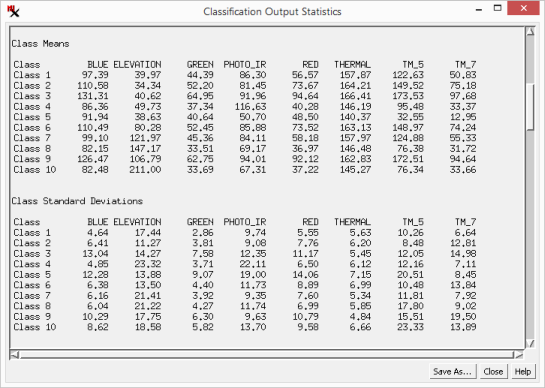
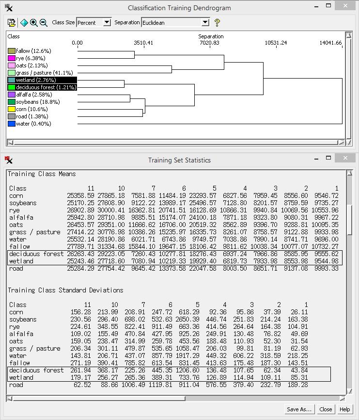
The ![]() Statistics icon opens a window that displays class statistics. This information enables you to investigate the spectral properties of each class and lets you compare classes for possible merging.
Statistics icon opens a window that displays class statistics. This information enables you to investigate the spectral properties of each class and lets you compare classes for possible merging.
Tabulated statistics include:
Class Counts - Number of cells and percentages for each class.
Class Means - Mean cell values of each class for every input raster.
Class Standard Deviation - Standard Deviation of each class for every input raster.
Class Distances between Means - Distance between Means for each possible class pairing.
Covariance matrix - Covariance Matrix
for each class gives a relative measure of the degree of spectral correlation for each possible
pairing of input rasters. High positive covariance values indicate a strong
positive correlation for the pair of rasters, values close to zero indicate little
correlation, and negative covariance values indicate a negative correlation between
the two rasters.
Start with a previous run of the process loaded so you see a class raster and classes listed. (I.e. load the class raster resulting from the first exercise.)
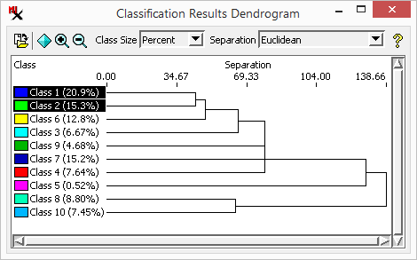
The ![]() Classification Dendrogram is a branching, tree-like plot that
shows the degree of spatial relatedness of the output classes. Class pairs that join together
near the left edge of the diagram are
closely related in their spectral properties and are thus good candidates for merging.
Classification Dendrogram is a branching, tree-like plot that
shows the degree of spatial relatedness of the output classes. Class pairs that join together
near the left edge of the diagram are
closely related in their spectral properties and are thus good candidates for merging.
The dendrogram process performs a successive grouping of pairs of classes, beginning with the pair having the closest class centers in spectral space as defined by the input bands. As each pair of classes is merged, a new joint class center is computed and class-center distances are recalculated. This process repeats until all classes have been merged into a single class. Results are plotted with the horizontal axis representing distance in spectral space with the degree of relatedness decreasing to the right. The vertical lines joining two classes are plotted at the distance that separated the corresponding class centers before the classes were combined.
The option lets you show class size as a percentage of cells or as cell counts (shown next to class name). The View menu provides options to zoom the x-axis scale on the dendrogram. and let you zoom in and out on the graph or display it fully. The option lets you save the dendrogram as a CAD object.
The option lets you choose a separability measure. The default is Euclidean, which shows the Euclidean distance between class centers in the feature space. Euclidean distance thus only depends upon the mean values of the classes. The other three choices (, and ) are statistical measures of the separation between classes that consider not just the class means but also the spread of values around the means. More specifically, they are computed for a pair of classes from the mean values and the covariance matrices. The distance increases continuously as the class means become farther apart in feature space, even beyond the point where there is no overlap between their distributions. The and measures have fixed lower and upper bounds, varying between 0 (classes have complete overlap) and 2 (no overlap). Both of these measures are also negative exponential functions of the distance between classes, so more weight is given to the difference between means for nearby classes.
separation - Distance in spectral space. Lower numbers mean classes are closer to each other.
Start with a previous run of the process loaded so you see a class raster and classes listed. (I.e. load the class raster resulting from the first exercise.)
Often classes you want to merge are near each other both spatially (as seen in the ) and spectrally (as seen in the dendrogram).
Alternatively, use the icon in the main process window to combine the classes.
Notice the dendrogram is updated along with the list of classes. Remember to manually save the updated class raster if you want to keep your changes.
The ![]() Confusion Matrix tool is used to compare the current class raster to another class raster in order to evaluate classification accuracy. You might compare the raster to the training set raster used to create it, another ground truth raster, or even to another class raster made using different methods or settings. For example, it is often used to assess the results of a supervised classification where the class of each sample area cell is compared to the class assignment produced by the supervised classification.
Confusion Matrix tool is used to compare the current class raster to another class raster in order to evaluate classification accuracy. You might compare the raster to the training set raster used to create it, another ground truth raster, or even to another class raster made using different methods or settings. For example, it is often used to assess the results of a supervised classification where the class of each sample area cell is compared to the class assignment produced by the supervised classification.
current class raster / result raster - Results of a classification run or a class raster re-loaded (via icon). It is automatically loaded in the . The current raster classes are shown when in mode in section of the main dialog window.
- The training set raster that was used to run a supervised classification. After running a supervised classification, the is automatically set up to compare the classification results with the training set raster used.
- Select another class raster such as a ground truth raster or another previously made class raster.
Tip: This analysis tool requires both rasters have matching classes. This is automatically true when you are comparing the resulting class raster of a supervised classification to the training set raster used.
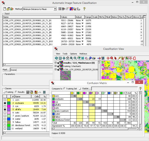
The matrix is organized with a column for each class in the class raster (cell value shown); likewise, there is a row for every class in the or (class name shown) you are comparing it to. This makes a bin for each possible pairing. The bins hold the class counts for any of the raster pixels that are classified in both class rasters. For each raster pixel, the class(es) assigned in both rasters are found, and the corresponding matrix bin is incremented by one. A glance at the matrix reveals the matching class pixel counts (gray diagonal) and non-matching pixel counts (non-gray bins) — in other words, correctly classified cells versus incorrectly classified cells. In other words, the gray background bins hold the number of correctly classified pixels in each class. Likewise, the values in off diagonal matrix cells represent misclassified (or differently classified) pixels.
In addition, total counts are computed for each column and row. The total count lets you compare the number of times a class is correctly predicted (gray diagonal) to the total number pixels in that class — the difference is the number of times it is misclassified.
- Total sample cell counts for both columns (output raster classes) and rows in the raster are figured.
In the above illustration, we are looking at what happens to the cells in the training set raster (rows) after you run the classification. Note, class raster totals are limited to the cells that have assigned classes in both rasters.
The bin values and totals are also shown as percentages for both the raster and the raster. In this way, two measures of accuracy are shown for each individual class: producer's and user's accuracy:
/ producer's accuracy - Values less than 100% indicate errors of omission ( raster cells omitted from the raster class). This is figured as the percentage of the diagonal bin value over the column . Non-diagonal bins in that column hold counts for cells that should be in that class (i.e. should be added to the training set samples).
Accuracy values for each column ( raster) indicate the percentage of cells of that class in the raster that were set to the same class in the raster.
/ user's accuracy - Values less than 100% indicate errors of commission (cells incorrectly included in the raster class). This is figured as the percentage of the diagonal bin value over the row . Non-diagonal bins in that row hold counts for cells that do not belong in that class (i.e. should be removed from the training set samples).
Accuracy values for each row ( raster) indicate the percentage of cells in the raster class that had the same class in the raster.
- Measure of agreement corrected by chance. A negative Kappa means that there is less agreement than would be expected by chance. See also: Cohen's kappa in Wikipedia.
Tip: Look for low percentage values and follow that row or column to find high cell counts in a non-diagonal bins. Look at the two associated classes for possible modification in the training set. Follow it up to find the raster class — add samples to the training set for this class. Follow it to the left to find the class — study the samples areas assigned to this class in the training set to see if you should remove some cells from those samples.
Training Set Error Matrix - A confusion matrix created using the training set raster. Because the raster cells in training areas are used to train a supervised classifier, classification accuracy is usually higher for these sample cells than for other areas in the scene.

Ground Truth Error Matrix - A confusion matrix created using the a separate ground truth raster that was not used for training. To get a better idea of the broader classification accuracy, you can use a second set of ground truth areas that were not used in the training set.
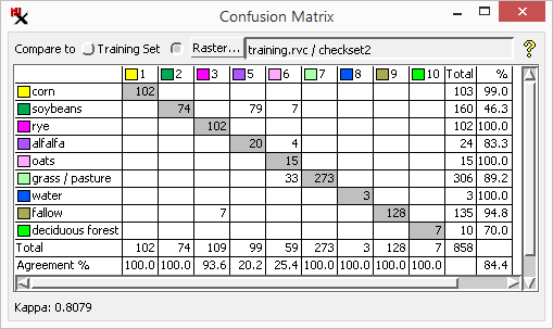
Open the confusion matrix for the training set raster; do the same for a different ground truth raster.
This exercise requires two ground truth rasters: one to be used as the training set and the other to check classification accuracy afterward. Set up for this exercise by running a supervised classification (i.e. Stepwise Linear with stanton_landsat8.rvc input and training.rvc/checkset1 as the training set).
The matrix opens showing a raster class in each row and a training set class in each column.
Note the Agreement % is generally higher with the training set than for the other ground truth raster.
This means some soybean cells in the training set raster were classified as alfalfa in the class raster. You can verify there is some overlap in the spectral properties of soybeans and alfalfa via and .
overall accuracy - Value calculated by dividing the total number of correctly classified raster cells (the sum of the leading diagonal values) by the total number of cells in the ground truth raster, and expressing the result as a percentage.
Keep in mind that the confusion matrix shows classification accuracy only relative to the set of classes that you provide. Low accuracy values for a particular class may indicate that the sample areas you used are not completely representative of the class, the class is not sufficiently different from other classes in its spectral properties, or your set of classes does not include all of the significant materials in the scene.
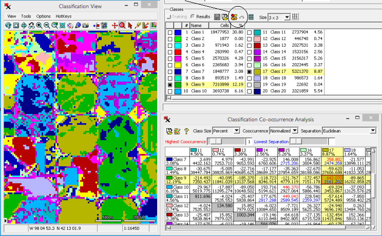
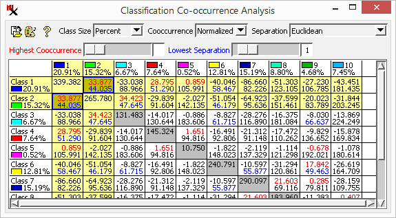
The ![]() Cooccurrence window is a matrix with bins holding both the spatial cooccurrence value and the spectral separability value for each pair of classes in the matrix cells. (Class names and sizes are listed on the horizontal and vertical axes. The option lets you show class size as a percentage of cells or as cell counts.)
Cooccurrence window is a matrix with bins holding both the spatial cooccurrence value and the spectral separability value for each pair of classes in the matrix cells. (Class names and sizes are listed on the horizontal and vertical axes. The option lets you show class size as a percentage of cells or as cell counts.)
cooccurrence (upper number) - The (raw or normalized) frequency with which cells of each class pair occur spatially adjacent to each other in the image. Higher numbers indicated classes frequently occur next to each other in the image.
The cooccurrence procedure analyzes the spatial associations of pairs of classes and the values shown allow you to judge which classes are spatially associated. These values are produced by comparing the raw frequencies of adjacency with
the values expected from a random distribution of
class cells, a calculation that removes bias related to
differing class sizes. A positive value indicates that
two classes are adjacent to each other more often
than random chance would predict. A negative value
indicates that two classes tend not to occur together.
The cooccurrence value shown by default is
the frequency, which adjusts the raw adjacency frequencies to remove the bias related to differing class sizes. Set the option to to see the raw frequency values.
separation (lower number) - Distance in the n-dimensional feature space defined by the image bands. Lower numbers mean classes are closer to each other.
The separation procedure analyzes the degree of spectral distance of class pairs. This is the same as figured for the dendrogram — see the Classification Dendrogram section for related information including options (, and ).
Classes with both high cooccurrence and low separation are good candidates for merging. Values are shown in color for the 10 values (red) and the 10 values (blue). The corresponding sliders let you find the matrix cell with highest/lowest cooccurrence/separation values respectively. When a slider is changed, the display automatically scrolls to the corresponding class pair and outlines the matrix cell in the same color.
- Classes with high cooccurrence values are near each other spatially.
- Classes with low separation values are near each other in spectral space.
The window is a quick and intuitive tool to analyze, select and merge classes. You can study both spatial and spectral relationships between the classes. The dialog provides shortcuts to merge classes — select/unselect classes by clicking on a matrix cell then merge selected classes via right-clicking on the matrix.
Start with a previous run of the process loaded so you see a class raster and classes listed. (I.e. load the class raster resulting from the first exercise.)
Notice how the value on the axis is where the vertical line joins the horizontal lines for the two classes.
Notice the yellow background and also that the two associated classes are selected in the main process window and other analysis windows.
Alternatively, use the icon in the main process window to combine the classes.
In practice, you may look for classes to merge where the matrix cell indicates both high cooccurrence and low separation.
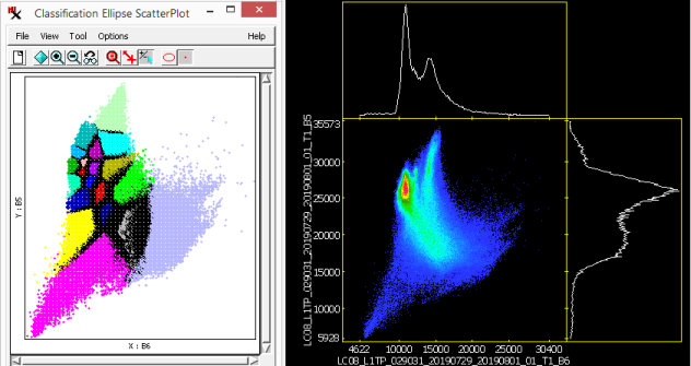
The ![]() Ellipse Scatterplot window shows the distribution of classes in spectral space projected onto a 2D plane in N-dimensional spectral space. You determine which two bands to look at by assigning them to the X and Y axes of the graph — a 'slice' of N-dimensional space. The positions of class clusters in spectral space can provide important information about the identity of the materials in each class. For example, a scatterplot of photoinfrared versus red bands is useful for recognizing classes representing bare soil, vegetated areas, and water. In addition, highly overlapping classes in multiple bands may indicate similar materials. You can view several spectral planes at the same time by opening more than one Ellipse ScatterPlot window.
Ellipse Scatterplot window shows the distribution of classes in spectral space projected onto a 2D plane in N-dimensional spectral space. You determine which two bands to look at by assigning them to the X and Y axes of the graph — a 'slice' of N-dimensional space. The positions of class clusters in spectral space can provide important information about the identity of the materials in each class. For example, a scatterplot of photoinfrared versus red bands is useful for recognizing classes representing bare soil, vegetated areas, and water. In addition, highly overlapping classes in multiple bands may indicate similar materials. You can view several spectral planes at the same time by opening more than one Ellipse ScatterPlot window.
Each class is represented by a scatter of cell values and/or the ellipses surrounding them. Both ellipse and points are drawn in the class color. However, when plotted points are dense or overlapping, black dots represent multiple classes. Ellipses for any classes selected (in the section of the main process window) are drawn with a dark gray fill color.
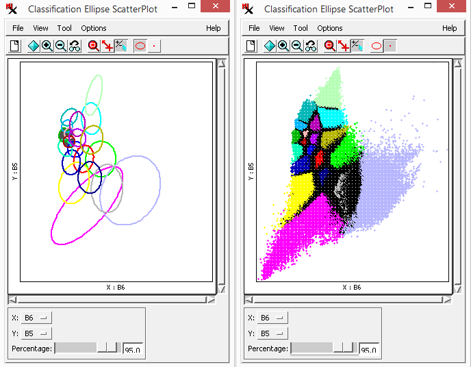
Use the slider to specify how many points ellipses are drawn around. The greater the percentage value the more encompassing the ellipse is; smaller (less encompassing) ellipses are drawn when a smaller percentage value is set. Adjust the plot using various options (via menu and toolbar) including: , , , and . The following tools are available as well: , , and .
It is difficult to imagine classes in the full N-dimensional spectral space (where N is the number of bands), however, the gives you a way to visualize class points by plotting them in two dimensions.
Start with a previous run of the process loaded so you see a class raster and classes listed. (I.e. load the class raster resulting from the first exercise.)
The selection tool in the window is not ideal — notice that all ellipses that overlapped the position you clicked on were selected along with their corresponding classes.
Tip: use the window to find the two classes with the lowest Separation value, which means they are closer to each other in spectral space than any other pair of classes. Note, it is easier to find related classes using the or another analysis window. It is also easier to select classes there or via the main dialog.
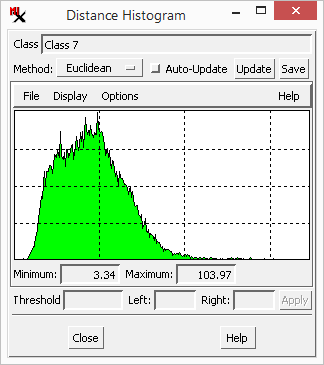
The ![]() Distance Histogram can help you assess the distribution of class points in spectral space for any class. It is derived from the distance raster that was automatically created for the current set of classes. Thus the graph plots the distance values of the last selected class. A compact class with a small spread of cell values has a narrow distance histogram. A diffuse class with many points far away from the class center has a histogram with a 'tail ' extending to higher distance values, or perhaps even a second mode (peak) in the
histogram. These outlier cells may represent distinctly different materials than cells near the class center.
Distance Histogram can help you assess the distribution of class points in spectral space for any class. It is derived from the distance raster that was automatically created for the current set of classes. Thus the graph plots the distance values of the last selected class. A compact class with a small spread of cell values has a narrow distance histogram. A diffuse class with many points far away from the class center has a histogram with a 'tail ' extending to higher distance values, or perhaps even a second mode (peak) in the
histogram. These outlier cells may represent distinctly different materials than cells near the class center.
You can remove outliers from the class by clipping the histogram tail. Set the distance to split the histogram and automatically update the percentage of points to the and of it. Or click and drag crosshairs in the histogram graph to do the same. your settings to clip the class value range and update the class raster accordingly. Discarded cells are assigned a 0 value in the class raster and will not be assigned to a class. Note that there is no way to undo this operation.
Choose the to graph (in the main process window) and then set the to compute the distance (Euclidean, Orthogonal, or Mahalanobis). Turn on to automatically recompute the distance histogram when you select a new class or manually it.
The graph has a menu that lets you create a of it or the histogram to a text file. The menu lets you choose how to display graph (Bar, Outline, or Strip). Set graph (for Grid, Logarithmic Scale, Cumulative, Show Transparent, Labels, and Label Size. The and histogram values are shown below the graph.
To try it out: select a class, click and drag crosshair position to set the distance , click to discard points above the threshold, and check the class raster in the for updated (null) areas.
Start with a previous run of the process loaded so you see a class raster and classes listed. (I.e. load the class raster resulting from the first exercise.)
It is important to know that any changes to the currently loaded raster are permanent. Thus saving a backup copy of the raster may be useful if you don't like your changes.
Notice that this sets the value.
Tip: in this exercise we removed an overly large portion of the cells in the selected class, however, in practice you would only cut off outlier values indicated by the histogram 'tail'.
Supervised classification methods require detailed knowledge of a portion of the study area so that you can designate sample areas for each of the desired output classes. These sample areas are used to train the classification algorithm. The training set raster should incorporate as much of the spectral variability in the scene as possible. Supervised classification methods determine the statistical properties of each of the training classes, then use these properties to classify the entire image.
Most of the supervised classification methods assign every non-masked input cell to one of the designated classes. If you identify too few training classes, the resulting class raster may be made up of "super classes" that have different features placed in the same class.
training set raster - Identifies representative sample areas for each of the desired output classes.
mean values vector (mean vector) - Directional line segment in N-dimensional space consisting of the mean values taken from each coordinate axis (variable). Here, the mean value vector represents the class centers of the set of input rasters plotted in spectral space.
feature space - The spectral space defined by classes in the training set raster.
The following supervised classification methods are available:. See the Supervised Methods and their Parameters section for details.
Running a supervised classification has the additional step of selecting a training raster.
The supervised classification exercises use data in stanton_landsat8.rvc for input and stanton_training.rvc for training and ground truth data.
Before running a supervised classification, a training set raster must be set up. Either select an existing training set raster, import it from vector training data, or manually create one using training data as a reference. Pixel values for each class in the training set are used to determine the class in the class raster. This section discusses the mode of the panel in the main process window, which has tools to create and work with a training set raster.
training data - Any type of information you may have about the ground cover or material in the study area that you want to use to 'train' supervised classification method being used.
training set raster (or layer) - Is a specialized class raster that contains class information for small portions of the study area. These sample classes are set up manually (or imported) for areas with known ground cover or material (i.e. ground truth information). As with other class rasters, each cell value in a training set raster represents a class. If classes are named, a database table is used to associate it with the correct cell value.
Tip: In regards to the loaded training set, pay attention to whether you are working with a temporary layer or a saved raster.
When you first create , the training set layer that is added is temporary. It must be saved to a raster in an RVC file (via ) to be able to the process or re-use the training set data later. On the other hand, any previously saved training set raster that is loaded will automatically retain any changes you make to the class list or assigned sample areas.
When mode is on in the section of the process, the following toolbar options are available.
Use to manage the training set 'raster':
![]() New Training Data - Creates a new temporary training set layer, which is initially a blank raster having no classes. You will need to set up classes by importing a class list or setting them up manually. You can then select a class and mark the sample areas in the using the tool along with information you know about the scene. This training set raster will not be saved until you use . After saving you can then the process.
New Training Data - Creates a new temporary training set layer, which is initially a blank raster having no classes. You will need to set up classes by importing a class list or setting them up manually. You can then select a class and mark the sample areas in the using the tool along with information you know about the scene. This training set raster will not be saved until you use . After saving you can then the process.
![]() Open Training Data - Open a previously saved training raster. It is automatically added to the and any changes you make to the raster or classes are automatically saved.
Open Training Data - Open a previously saved training raster. It is automatically added to the and any changes you make to the raster or classes are automatically saved.
![]() Save Training Data As - Saves the currently loaded training set (either a temporary layer or saved raster) to a new raster object in an RVC file. Note, any temporary training set layer you make must be saved this way before you can the process. On the other hand, there is no need to save a training set raster after editing since it is saved automatically as you go.
Save Training Data As - Saves the currently loaded training set (either a temporary layer or saved raster) to a new raster object in an RVC file. Note, any temporary training set layer you make must be saved this way before you can the process. On the other hand, there is no need to save a training set raster after editing since it is saved automatically as you go.
![]() Edit Training Data - Toggle mode to allow editing the currently loaded training set raster. When this button is on you can modify training set classes (name, cell value, and color). This mode is off by default after loading a saved training set raster. This is a safety measure since modifications are saved automatically and you cannot revert back to the original.
Edit Training Data - Toggle mode to allow editing the currently loaded training set raster. When this button is on you can modify training set classes (name, cell value, and color). This mode is off by default after loading a saved training set raster. This is a safety measure since modifications are saved automatically and you cannot revert back to the original.
Tip: Instead of turning on the mode, use to create a new training set raster (with mode on automatically). Then you can make changes without modifying the original training set raster.
![]() Import from Vector - Imports polygon or point vector data to a training set raster and loads the resulting training raster.
Import from Vector - Imports polygon or point vector data to a training set raster and loads the resulting training raster.
Note, if you don't have a training set raster loaded, a new temporary training layer will be added. However, if you already have a training set raster loaded the imported training areas and classes will be merged with it. The mode must be on if you want to import / merge into a loaded training set raster.
Use to manage class list:
![]() Open Class Table - Creates a temporary training set layer with classes specified by the table. You can select any class table previously created via . If a training set raster is already loaded you will have the option to merge the new classes with the current class list ().
Open Class Table - Creates a temporary training set layer with classes specified by the table. You can select any class table previously created via . If a training set raster is already loaded you will have the option to merge the new classes with the current class list ().
![]() Save Class Table - Save the current class list (class numbers, names, and associated colors) to a new table in an existing database. User can navigate into a class raster such as the current training set raster, a vector object such as point or polygon training data, or a main level database object.
Save Class Table - Save the current class list (class numbers, names, and associated colors) to a new table in an existing database. User can navigate into a class raster such as the current training set raster, a vector object such as point or polygon training data, or a main level database object.
This option lets you to make and use a consistent set of classes and colors for related datasets. This table can be reopened later in the Training Set Editor via .
![]() Add Class - Add a new class to the current class list.
Add Class - Add a new class to the current class list.
![]() Delete Selected Class - Deletes classes that are currently selected via a filled selection box. This option is active when toggle is on. Sample areas of that class will be removed from the raster as well unless you use that cell value in a new class.
Delete Selected Class - Deletes classes that are currently selected via a filled selection box. This option is active when toggle is on. Sample areas of that class will be removed from the raster as well unless you use that cell value in a new class.
Use to manage updated cell values assigned to classes (modifies both training set 'raster' and class list):
![]() Apply Cell Value Changes - Updates the training raster to match the modified cell values in class list.
Apply Cell Value Changes - Updates the training raster to match the modified cell values in class list.
Tip: Turn on mode to modify classes.
![]() Reset Cell Value as Saved (Undo) - This reverts the class cell value(s) to the state prior to edits. In other words, the class list reverts to match the training raster as displayed in the .
Reset Cell Value as Saved (Undo) - This reverts the class cell value(s) to the state prior to edits. In other words, the class list reverts to match the training raster as displayed in the .
When a supervised classification method is chosen, the panel is automatically set to be in mode, which is then used to create, open, or import a training set raster. Once a training set raster is loaded the and toolbar options become active, which provide statistics for the training set classes. This information can be used to judge the spectral characteristics and separability of the training classes.
After running a supervised classification the panel is automatically switched to mode and all of the analysis tools are available to study the raster. Furthermore, if you open the it will be automatically set up to compare the resulting classes to the training set.
Set up by selecting a supervised classification method (i.e. ) and loading input (stanton_landsat8.rvc) and training set (stanton_training.rvc, training_raster).
For detailed setup instructions see the exercise.
See the Confusion Matrix (Error Matrix) section for more information on using it to analyze class accuracy.
Use the icon to convert vector polygons or points containing ground truth information (elements with attributes) to a training set raster. Objects to be used for importing training areas must be georeferenced, but need not match the extents of the input. The new training set raster is automatically co-aligned with the input rasters, and thus only transfers training areas in the overlap area.
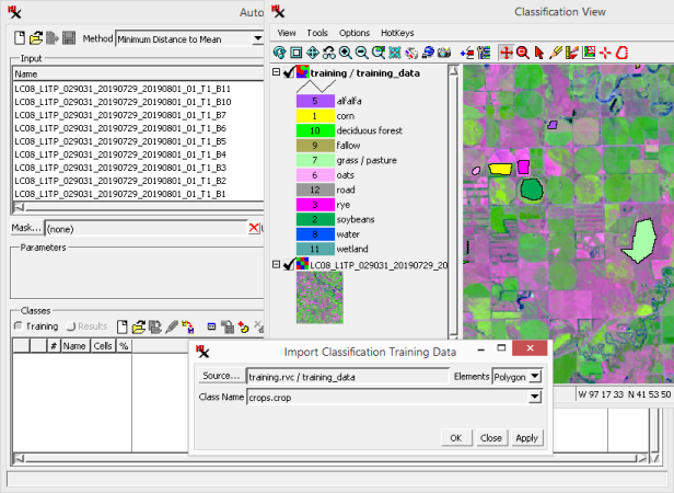
Create a training set raster by importing from a polygon or point vector.
Close the process and re-open it to start fresh. Set up a supervised classification with input: stanton_landsat8.rvc file and method: . Ground truth objects are in stanton_training.rvc.
A new temporary training set raster is automatically created (unless one was previously loaded).
Notice the vector is shown in the while you have the set in the dialog.
Note the updated value for the selected class in the main dialog.
The above steps show how you can interactively import one class at a time. The next steps show you how to import many classes at once.
Note, the table specified is in the vector's polygon database. The table has records for each class containing a style color, the class name, the and the class number.
Note that any previously set classes and samples in the training set may be retained as-is or overwritten when you import. That is why you still see the class you added manually in the first step of this exercise, however, the value is now 0 because a polygon used in the last step covered the same area.
Notice the icon becomes available after saving the new training set raster.
Try it with vector points: repeat the above steps except choose a point vector (stanton_training.rvc / training_points with crops.crop table and field); set to 20; and click .
Note, if you already have a training set raster (or temporary layer) loaded, the new classes and class samples will be automatically merged with it. (You will need to turn on to do so with a saved training set raster.)
Tip: use to interactively import classes to the training set one at a time. Use to automatically close the dialog after importing.
If you don't already have a training set raster or importable ground truth data, you can create a training set raster manually within the process. You will set up the class list and add samples using a reference layer such as a map with hand drawn ground truth information or a raster layer with high enough resolution that you can recognize features.
When creating a training set raster manually, you may decide to set up the class list first or as you add samples. Use the option to manually create the class list. Or import them if you have previously set up a class list for another training set raster or have named classes in a previously made class raster. Using a table to store class information is useful because it lets you use re-use the same class names, cell values, and color palette when running multiple supervised classifications for the same or related datasets.
You can import a class list from a table that is stored in a main level database object or under a class raster. Note, a class raster will only have a database table if classes were manually named. A class list table in a training set raster can be saved to a main level database object for later use.
Open a previously saved class list. Learn how to modify and save it.
Close the process and re-open it to start fresh.
Notice a new, empty training set raster is automatically created and added as a layer in the . This is a temporary raster but you will be prompted later to save it to an .rvc file.
Also notice, the icon is automatically turned on.
Note, you could have added all the classes this way instead of starting with the imported class list.
With a class list and an empty training set raster loaded, you can start drawing samples as shown in the next lesson.
Tip: if you already have a class list loaded and use , you will be prompted to If you choose the new classes will be merged with the previously loaded class set.
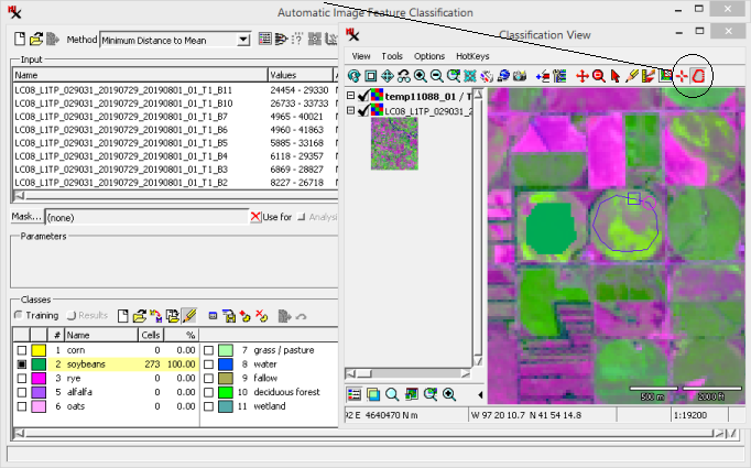
The steps to add a sample to be used for training are: select a single class, draw the sample area, and choose an assignment option. In this way classes are assigned to each sample as you drawn them in the .
A typical operation would involve first finding an area in a reference layer that is made up of a single class. Select that class in the usual way from the list in the main process window. Then turn on the tool, which is at the right side of the top toolbar in the . This activates the standard polygon drawing tool so you can draw a polygonal shape outlining the sample area. Finally, when the polygon is drawn, right-click on it and choose an assignment option from the menu that opens, thereby associating it with the selected class.
Assignment options include:
- All cells in the polygon that do not yet have a class assignment are added to the selected training class.
- All cells in the polygon are added to the selected training class regardless of previous class assignment.
- All cells in the polygon are marked as unclassified.
- All cells of the selected class (or classes) become unclassified.
- Select class(es) by moving mouse over the class samples in the . The drawn polygon limits classes that can be turned on.
- Unselect class(es) by moving mouse over the class samples in the . The drawn polygon limits classes that can be turned off.
- Toggle whether class(es) are selected or not by moving mouse over the class samples in the . The drawn polygon limits classes that can be toggled.
Note, once you have sample areas added to the ground truth raster, the icon in the top toolbar of the can also be used to select a class.
(continued from previous exercise)
Add class samples to a new training set raster.
You can start where the previous exercise left off. Or, set up a supervised classification with a class list and empty training set raster (input: stanton_landsat8.rvc, method: Suits Maximum Relative, class list: training.rvc, class_database object, CLASSINFO table).
Notice after adding samples for two classes, the Save Training Data As icon becomes available.
Tip: the method only classifies raster cells that fit within the class criteria and thus the resulting class raster has null areas. Increase the to classify more raster cells.
See the Supervised Classification section for information about using a training set raster when running the process.
See the Unsupervised Classification section for general information about using an unsupervised classification method. The following parameters are used in all unsupervised methods:
- sets an upper limit on the number of output classes. Increasing the output class limit also makes it more likely that similar cover types will be assigned to distinct classes rather than being lumped together in a single class.
- Sets an upper limit on the number of
iterations performed in the class building
phase of the process.
The following parameter is used with the and methods:
- sets the threshold distance in spectral space used to designate an input cell as a new class center instead of assigning it to the closest class. By adjusting this parameter downward, you increase the likelihood that different land cover types that are close together in spectral space will be assigned to distinct classes.
The following parameters are used with the and methods:
- A class center is considered to be steady when its movement with successive iterations falls below this value.
- Sets the percentage of class centers that must become steady in order to accept the current set of classes.
The method analyzes the input raster set to determine the location of initial class centers. In each process iteration, cells are assigned to the nearest class and new class centers are calculated. The new class center is the point that minimizes the sum of the squared distances between points in the class and the class center. With each iteration, class centers shift and the class assignments for some cells change. The process repeats until the shift in class centers falls below a specific value or the maximum number of iterations is reached.
The method uses rules of fuzzy logic, which recognize that class boundaries may be imprecise or gradational. The Fuzzy C Means method creates an initial set of prototype classes, then determines a membership grade for each class for every cell. The grades are used to adjust the class assignments and calculate new class centers, and the process repeats until the iteration limit is reached.
The Fuzzy C-Means method is slower than other methods (such as KMeans) so for large datasets you may want to set the option to use a subset (sampling) of the input.
The method uses an iterative approach to compute classes. The algorithm uses the set of values for each input cell to define a vector in feature space. The process analyzes the sample dataset to determine class centers, using the differing angles between sample vectors (distribution angles) as a measure of relatedness. Sample vectors separated by small distribution angles are assumed to be more closely related than those with larger distribution angles. The algorithm re-analyzes the angles using the results of the previous iteration to determine improved cluster centers. The process can create an optional distance raster.
The method is similar to the K Means method but incorporates procedures for splitting, combining, and discarding trial classes in order to obtain an optimal set of output classes. The ISODATA method determines an initial set of trial class centers and assigns cells to the closest class center. In each subsequent iteration the process first evaluates the current set of classes. A large class may be split on the basis of its number of cells, its maximum standard deviation, or the average distance of class samples from the class center. A class that falls below a minimum cell count threshold is discarded, and its cells are assigned to other classes. Pairs of classes are combined if the distance between their class centers falls below a threshold value. After classes have been adjusted, new class centers are calculated and the process repeats. Process iterations continue until there is little change in class center positions or until the iteration limit is reached.
- The Minimum Cluster Cells parameter sets the lower limit for the number of cells in a class. Any class with fewer cells is dissolved, and its cells are reassigned to other classes.
- The Maximum Standard Deviation parameter provides one criterion for splitting large classes. If the class standard deviation for any input band exceeds this value, the class is split into two classes.
- The Minimum Distance to Combine parameter sets the threshold distance used to determine if two nearby classes should be combined.
- The Minimum Distance for Chaining parameter applies to the initial creation of class centers. It sets the lower limit on the distance between two class means.
The method is based on neural network computing techniques. Neural network learning is the process of adapting connection weights in response to sets of input values and resulting sets of output values. The Self Organization neural network is designed to recognize natural groups of spectral patterns in a sample of the input data, and to produce a consistent neural net output (class identification) in response to input of similar patterns during classification of the entire image.
The neural network used in the Self Organization process is a three-layer net in which the middle (hidden) layer consists of nodes arranged in a two-dimensional matrix. The initial values of connection weights between input nodes and hidden layer nodes are set randomly. As sample input data are fed to the neural network during the learning phase, connection weights are modified using a competitive learning strategy.
The set of raster values associated with a single cell in the sample input can be considered to be the coordinates of a position in feature space. These values are fed to each node in the hidden layer, where they are compared to the current set of weights for the node. The node with the closest match to the current position in feature space is determined on the basis of minimum Euclidean distance. The winning node and nodes in a surrounding local neighborhood have their weights updated to reduce the error in matching, while other nodes remain static. With successive iterations of the sample data, different neighborhoods in the hidden layer are trained to recognize specific classes of input pattern. Connections between the hidden and output layers are modified so that the net produces the same output if any of the nodes in a particular neighborhood is activated. The learning phase continues until the conditions established by the user-defined parameters are met. The trained neural net is then used to classify the entire input image. The process can create an optional distance raster.
The method is based on neural network computing techniques that is designed to recognize natural groups of spectral patterns in the input data, and to produce the same neural net output (class identification) in response to input of similar patterns.
Neural network learning is the process of adapting connection weights in response to sets of sample input values and resulting sets of output values. The initial values of connection weights between input nodes and hidden layer nodes are set randomly. Like the method described above, the method uses a competitive learning strategy to update connection weights.
Some competitive learning models do not produce satisfactory classification results with highly variable input. This can occur because training in response to later input patterns can undo the effects of training that occurred earlier in the learning phase. The classification method uses a complex neural net architecture to ensure both stability and plasticity in response to widely varied training input. As in the Self-Organization method, the learning phase consists of multiple iterations of the sample data, which train different neighborhoods in the hidden layer to recognize specific classes of input pattern. The Adaptive Resonance algorithm includes tests to ensure that an existing neighborhood is only modified if the current input pattern is sufficiently similar to the average pattern for that neighborhood (Euclidean distance is used as the measure of similarity). If the current input vector passes this test, the closest matching node in the neighborhood is activated, its weights are updated to reduce the mismatch, and the average pattern for the neighborhood is updated. Otherwise, the closest matching node outside of existing neighborhoods is activated, and is used to form the nucleus of a new neighborhood (thus creating a new output class). The learning phase continues until the conditions set by the user-defined parameters are met. The trained neural net is then used to classify the entire input image. The process can create an optional distance raster.
See the Supervised Classification section for general information about using a supervised classification method. The following supervised classification methods are available:
The method first analyzes the class areas designated in the training set raster, then calculates a mean value in each input raster for each training class and thus defines the class center in spectral space (mean values vector). The process then assigns each cell in the input raster set to the class with the closest class mean in spectral space.
The Minimum Distance to Mean algorithm is mathematically simple and efficient,
but it does not recognize differences in the variance of classes, which has to do with their relative size in feature space. Thus, training sets with classes having different variances that lie close to each other in feature space may result in miss-classification of data points near the edge of a large class that may be closer to the center of a nearby smaller class than to their own class center. For this reason, the method works best in applications where spectral classes are dispersed in feature space and have similar variance.
This method has no user-defined parameters. The user has the option to create a distance raster when setting output raster path and name.
The method applies probability theory to the classification task and can be thought of as a refinement of the method. So in addition to considering the distance from the class mean it also uses the relative size (variance) and shape (covariance) in spectral space. These statistics are then used to compute the probability that a given raster pixel belongs to a particular training set class. It computes all of the class probabilities for each raster cell and assigns the cell to the class with the highest probability value (maximum likelihood).
variance - A measure of how far a set of numbers is spread out. Specifically it is the average of the squared differences from the mean. Think of it here as the relative size of a training set class in feature space.
covariance - Indicates how two variables change together. Here a variable is the value of a coordinate along one axis in feature space. The covariance can provide information about the shape of the class in feature space.
mean values vector (mean vector) - Directional line segment in N-dimensional space consisting of the mean values taken from each coordinate axis (variable). Here, the mean value vector can be thought of as the class centers for a set of input rasters plotted in spectral space.
The probability that a pixel belongs to a particular class depends on the distance between it and the class center, and also on the variance and covariance of the class. The method interprets the cell values in each training set class as having a Gaussian (normal) distribution, which can be described by the mean vector and the covariance matrix.
- The probability values calculated by the Maximum Likelihood classifier in its default mode are based solely on spectral characteristics. But in some cases you may know independently that one class should be rare in the scene while another class should be very common. This prior knowledge could come from historical data (for example, records of the proportions of the area planted to different crops), or current information on similar areas.
A probability value based on such information is termed an a priori probability. The values can be percentages or between 0 and 1, but must be tabulated for each class in a single field in a database table attached to the training set raster. The a priori probability values are used as weighting coefficients in calculating class assignment probabilities.
- this threshold lets you exclude cells that don't fit any of the training classes particularly well. If the highest class probability for a cell is smaller than this threshold, the cell is not classified, and is assigned a value of 0 in the class raster.
The method produces more accurate class assignments than the method when classes vary significantly in size and shape in spectral space. However, it is computation-intensive and thus processing time is relatively long. Without a priori values, this method assumes that each class has an equal probability of occurring in the scene and thus may not be valid for remote sensing applications.
This method has no user-defined parameters and can create an optional distance raster.
The method uses linear discriminant analysis to define a new set of coordinate axes in feature space that most effectively differentiates classes, then projects input cell values into this coordinate system for classification.
discriminant functions - A set of derived variables that are linear combinations of the original variables. Each discriminant function can be visualized as a straight line in feature space.
linear discriminant analysis - A statistical technique that calculates a set of discriminant functions that separates classes.
variable - Refers to an input raster in feature space.
The method analyzes the training set and chooses the set of discriminant functions that produces the best possible separation (discrimination) between the classes in the training data. Discriminant functions are chosen using a stepwise procedure that selectively adds and removes input bands to find the minimum number of bands necessary to produce the optimal separation of training classes. In each step, an additional variable is selected for possible inclusion in the discriminant function and must meet certain requirements. Existing variables are also evaluated using removal criteria. Successive discriminant functions are constrained to be mutually perpendicular. This stepwise selection of variables terminates when no more variables meet the entry or removal criteria. Thus input rasters that do not add significantly to the discrimination of classes are eliminated from the classification process.
This method is particularly appropriate when you have a large number of input rasters as it minimizes the number of necessary bands. Also note, the possibility of assigning cells to the wrong class is minimized when variables are normally distributed within each class, and the covariance matrices are equal.
The user has the option to create a distance raster when setting output raster path and name.
The algorithm computes the composite brightness and the ratio of each band's brightness over the composite brightness. The algorithm calculates the mean and standard deviation of each of these parameters for the training class and uses them to define the class boundaries.
composite brightness - Sum of each individual band's values.
The algorithm calculates the composite brightness and band brightness ratio for each input cell, and assigns the cell to a class by comparison with the class boundaries defined from the training set. Unlike other methods, this method does not assign every non-masked input cell to a class. In contrast, it creates rigid class boundaries and leaves cells located outside the boundaries unclassified.
- This value scales the size of the class assignment partitions. A value greater than or equal to zero with precision to four decimal places can be entered; the default value is 2.0000.
This method has a computational speed advantage over other methods. Cells falling outside the boundaries of any class are left unclassified.
The user has the option to create a distance raster when setting output raster path and name.
The method is based on neural network computing techniques. Learning in neural network theory is the process of adapting connection weights in response to sets of input values and resulting sets of output values. Back propagation is a specific learning algorithm by which a multilayer neural network can be trained to recognize and classify spectral patterns as it processes the training set data. The goal is to adjust the network parameters so that it correctly classifies patterns from outside the training set as well
The set of raster values associated with a single cell in a training area can be considered to be mathematical components of an input vector. Each of these raster values is fed to a single node in the input layer of the neural network. The output layer of the network contains one node per class; the set of values produced by the output layer nodes in response to an input vector constitute an output vector. Learning via back propagation involves comparison of the output vector with the desired classification result, or target vector. The target vector has a value of 1 for the node corresponding to the correct training class, and 0 for all other nodes. If the output vector does not match the target vector, connection weights are adjusted to reduce the difference. The network is initialized by setting random weight values, or by using an additional learning algorithm to estimate initial weights. As the set of input vectors from a training set are fed repeatedly to the network, the back propagation algorithm adjusts the weights in each pass to minimize the squared error (difference between output and target values) over the training set. Iterations continue until the error in output values falls below a user-defined limit, or until the process reaches a specified number of iterations. Once the learning phase is complete, the trained neural network is used to process and classify the image.
- sets an upper limit on the number of iterations. The allowable range of values is 1 to 10000, with a default value of 10. The number of iterations needed to produce desirable results varies widely depending on the input. Changes made to the class centers may diminish to an insignificant amount after some number of iterations less than the specified maximum. For example, 95 percent of a center's changes may occur in the first twenty iterations and only three percent in the next twenty iterations. Increasing the Maximum Iterations parameter may improve classification results, at a cost of increased processing time.
- The parameter also controls the amount of the weight adjustment. The parameter is used to set the Maximum cumulative error allowed by the process.
- The parameter is a multiplying term used to control the adjustment of connection weights. The allowable range of values is 0.0000 to 1.0000; the default value is 0.9000. Increasing this value increases the rate of change in connection weights with each iteration, and thus increases the learning rate of the neural network.
- The Error Threshold parameter sets the error limit for terminating the training of the neural network classifier. When the current classification error rate of the neural network falls below the value set by this parameter (or the training process reaches the maximum allowable number of iterations), training is terminated. The allowable range of values is 0.0000 to 1.0000; the default value is 0.0100 (corresponding to 1% misclassification of training data).
The method is based on neural network computing techniques. Learning in neural network theory is the process of adapting connection weights in response to sets of input values and resulting sets of output values. Mahalanobis is a specific learning algorithm by which a multilayer neural network can be trained to recognize and classify spectral patterns as it processes the training set data. The goal is to adjust the network parameters so that it correctly classifies patterns from outside the training set as well.