
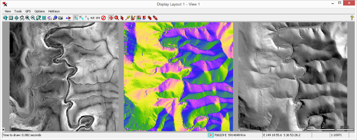
The process computes rasters with fundamental topographic property values derived from an input Digital Elevation Model (DEM) raster. Properties include: and .
selected, which is also is shown here in the process.
Prerequisite Skills: Getting Started and Displaying Geospatial Data.
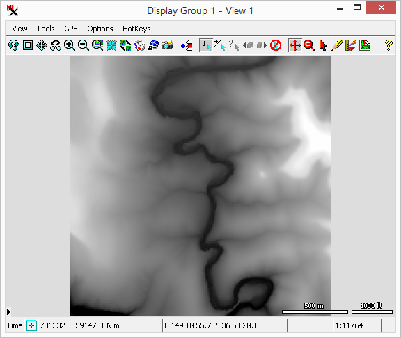
Sample Data: coolumbooka.zip
(A portion of a 2 meter DEM from NSW FSDF was extracted to fit within the size constraints of the TNTmips Free license level.)
Tutorial Lesson: One exercise provides a quick introduction (see below).
shown here with set to .
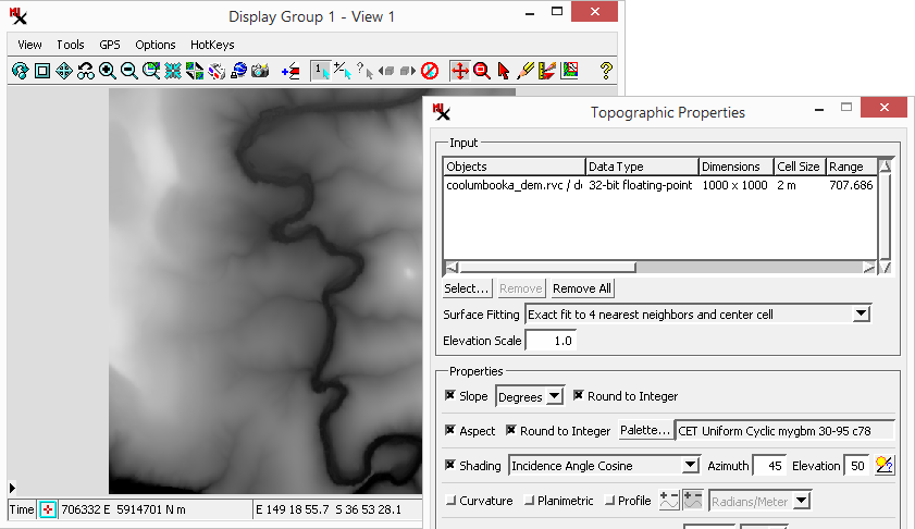
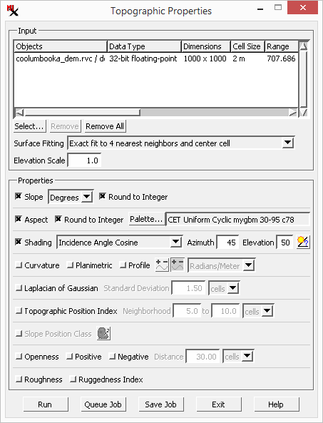
To run the process: select an input DEM, toggle on the you want to compute, then .
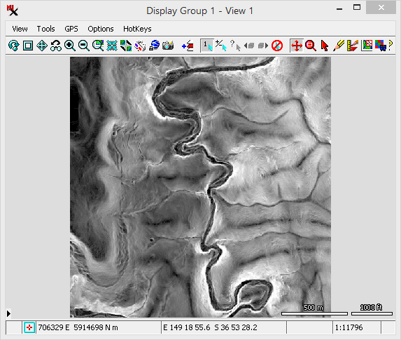
The process takes one or more elevation rasters as input (signed/unsigned integer: 8-, 16-, and 32-bit; floating: 32- and 64-bit).
(shown here in the process).
A separate output raster will be made for each property option turned on. Properties include: and and are described below.
The is a measure of the magnitude of surface steepness, which is computed as the vertical angle in degrees or as percent slope = 100 * tan (slope angle). You can set output cell values to: or as well as the option to .
The is the map direction of downward slope, expressed in degrees of azimuth angle (range 0 to 360 increasing clockwise from north). Flat areas are indicated by the value -1. You have a option for output cell values and the option to set the color palette used to display the resulting aspect raster.
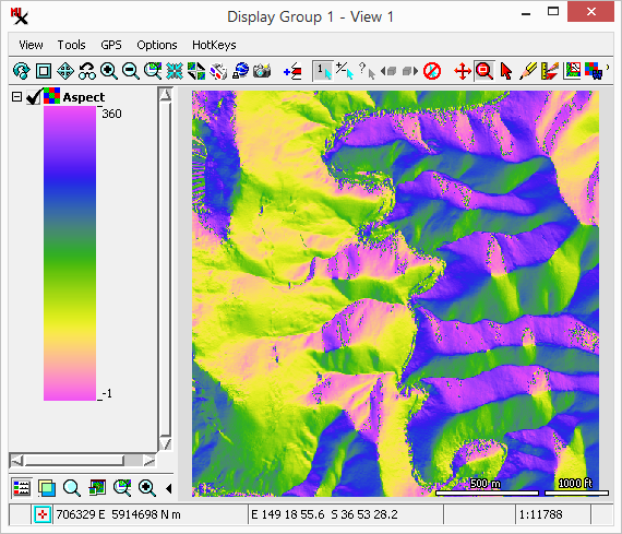
avoid discontinuities in the colors between 0 and 360 degrees.
TIP: The aspect and shading computations assume that the raster is oriented with north (the 0 azimuth direction) at the top. Raster objects that are not so oriented should be reprojected using the process prior to computing topographic properties.
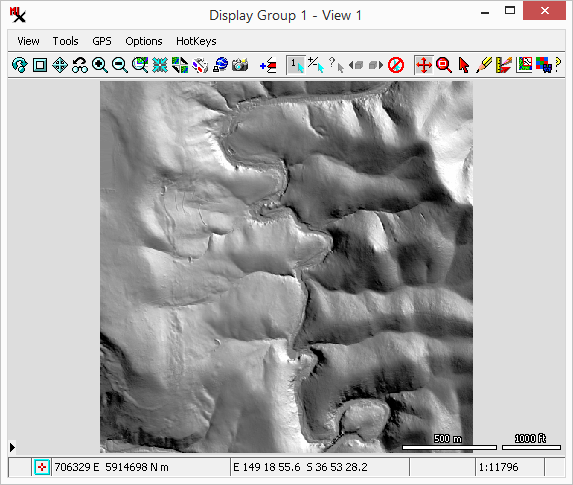
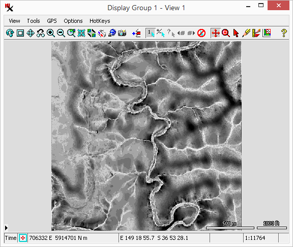
The option computes a shaded-relief image of the elevation surface assuming uniform sunlight from the specified sun elevation angle and compass direction (azimuth). The resulting brightness varies with the slope angle and aspect.
Three methods are available for computing shading brightness values:
method – uses the same algorithm as the option in the process.
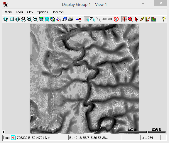
method – computes the cosine of the angle between the sun and the surface and the result will generally vary between 0 and 1. The scaled version of this method rescales the cosine range to span the 8-bit unsigned integer data range (0 to 255). When viewed, this will typically have a higher contrast than the method.
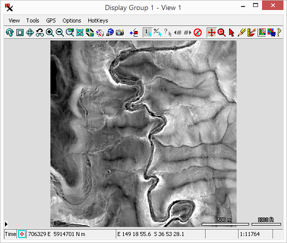
The and parameters specify the direction of the incoming light source / sun. Azimuth ranges from 0 to 360 degrees clockwise from north. Elevation is the angle above the horizon from 0 to 90 degrees. Additionally, the ![]() can be used to calculate these parameters.
can be used to calculate these parameters.
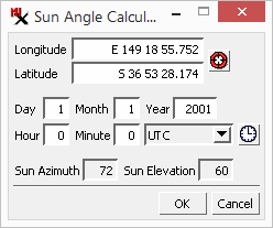
The automatically computes sun elevation and direction values for a particular geographic location, date, and time. You can use the calculator to produce a shading raster with illumination conditions approximating those of an aerial or satellite image with known acquisition date and time. Set the values in the and fields to specify the position. Set the (1-12) and fields to specify the date. Set the (0-24) and fields to set the time of day in Coordinated Universal Time (UTC). (UTC is sometimes referred to as Greenwich Mean Time, which is equal to the local time in the United Kingdom.)
TIP: The aspect and shading computations assume that the raster is oriented with north (the 0 azimuth direction) at the top. Raster objects that are not so oriented should be reprojected using the process prior to computing topographic properties.
The option computes the curvature of a line formed by intersecting the terrain surface with a horizontal plane () or vertical plane parallel to the local slope direction (). The computed value is the reciprocal of the radius of curvature of this hypothetical line, which can be computed in radians/meter or radians/100 meter. Larger curvature values indicate a smaller radius of curvature and thus a tighter, more pronounced curve. Curvature values can be computed in units of radians per meter (yielding very small values) or radians per 100 meters.
option - curvature values are positive for surfaces that are convex outward. Plan curvature is undefined for flat areas and a value of 0 will be output.
option - the user can choose whether curvature are  or
or  .
.
provides another measure of curvature in a local neighborhood. The neighborhood is based on the standard deviation value provided.
The option compares the elevation of each cell to the mean elevation of a specified neighborhood around that cell. Positive TPI values represent locations that are higher than the average of their surroundings, as defined by the neighborhood (ridges). Negative TPI values represent locations that are lower than their surroundings (valleys). TPI values near zero are either flat areas (where the slope is near zero) or areas of constant slope (where the slope of the point is significantly greater than zero). The designated neighborhood is usually a ring (annulus) over a range of distances. Cells near the edge of the DEM will have incomplete neighborhoods and so will be less accurate.
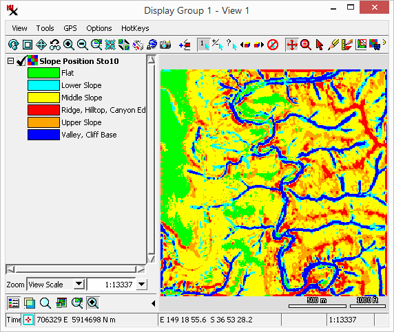
The option is based on and and thus requires them to be selected as well. This property classifies cells into Ridge, Upper Slope, Middle Slope, Lower Slope, Valley, and Flat classes. The user has the option to choose the colors used in the classification. For more information on TPI and SP classification see www.jennessent.com/downloads/tpi-poster-tnc_18x22.pdf.
expresses the degree of dominance or enclosure of a location on an irregular surface. The user can specify the distance over which the computation is performed. See Ryuzo Yokoyama, Michio Shirasawa, and Richard J. Pike, Photogrammetric Engineering & Remote Sensing, March 2002.
The is defined as the mean difference between a central pixel and its surrounding cells. is computed as the largest inter-cell difference of a central pixel and its surrounding cell. See Wilson et al 2007, Marine Geodesy 30:3-35.
The dialog includes an section to select the input raster(s) and the method. The section has toggles you can turn on for each of the output rasters you want to make.
Click the button to choose one or more input rasters. and let you remove one or more items from the input list.
The topographic properties are computed for each raster cell using the input elevation values in a 3 by 3 cell kernel centered on the current cell. Slope and aspect are computed from finite-difference approximations of the first derivatives in the column (x) and line (y) directions. Curvatures are computed using finite-difference approximations of the first and second derivatives in the x and y directions. Different combinations of the kernel cells can be used to compute these derivatives. Each of these combinations represents a different mathematical approximation or model of the shape of the local surface. The Surface Fitting menu provides a choice of five surface models.
– Uses only the four nearest neighbors of the center cell in the line and column directions to calculate the first derivatives for the slope computation. The diagonally-adjacent cells in the corners of the kernel are ignored. The center cell is used in combination with the four nearest neighbors to calculate the second derivatives for the curvature computation. The method is geometrically equivalent to a model surface that passes exactly through the center cell and its four nearest neighbors. It provides no averaging and thus no smoothing of noise that can arise from local errors in the elevation values.
– This method uses all eight neighbors of the center cell to calculate the topographic properties. Each of the first derivatives for the slope computation uses the average of three pairs of elevation differences across the kernel (three in the line direction and three in the column direction), and the second derivatives are computed in a similar fashion using the center cell as well. This method produces a local quadratic (second-order) surface that is a best-fit to the elevation values in the kernel, and is thus not constrained to pass exactly through each cell. This method produces a smoother local surface that is less sensitive to local elevation errors than the method. The remaining methods are variations of this method.
– This method uses all eight neighbors of the center cell to calculate the topographic properties. Each of the first derivatives for the slope computation uses the average of four pairs of elevation differences across the kernel, with the nearest-neighbor pairs of the center cell being counted twice. The second derivatives are computed in a similar fashion using the center cell value. This method weights the nearest-neighbor cells more heavily than the diagonally-adjacent cells in computing a best-fit local quadratic surface, with the weighting factor being inversely proportional to the square of the distance from the center cell.
– Uses all eight neighbors of the center cell to calculate the topographic properties. Derivatives are computed using a weighting factor equal to the square root of 2 for the nearest-neighbor elevation differences. This method weights the nearest-neighbor cells more heavily than the diagonally-adjacent cells in the computing the best-fit quadratic surface, with the weighting factor being inversely proportional to the from the center cell distance.
– Second derivatives are also computed in a similar manner as the method, but use a weighting factor of 3 for the center cell. This method produces a quadratic surface that is constrained to pass through the current (center) cell for purposes of curvature computation.
Adjust the to exaggerate or reduce the input range.
This section lets you choose which output rasters you want computed. Properties include: and . See the Results / Output section for details on each one.